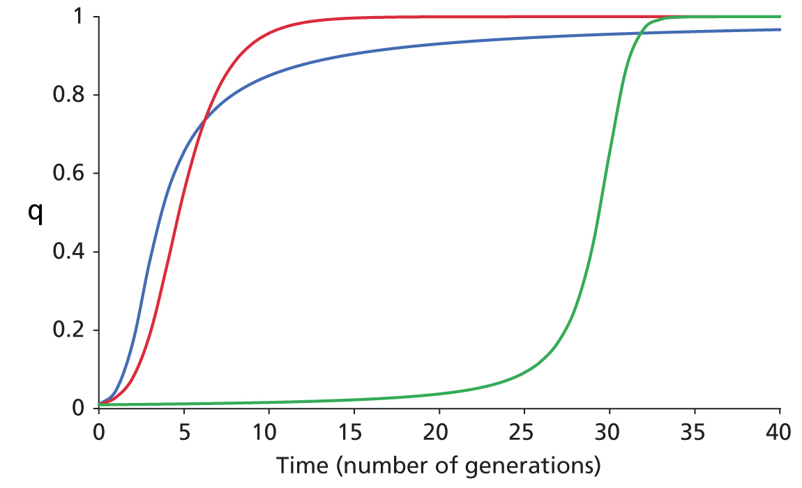
Change in frequency
of a rare allele under Positive
Directional Selection
Dominant, Additive Semi-Dominant, & Recessive cases
In a single-locus model
with two alleles A and B, let
initial q = f(B)
= 0.001. The three curves
trace f(B)
over time for three
modes of dominance.
The Blue curve
shows the case where B is dominant
to A (WBB
= WAB ![]() WAA). The Red curve shows an additive (semi-dominance) model, in
which each B
allele decreases fitness by the same amount, such
that WBB
WAA). The Red curve shows an additive (semi-dominance) model, in
which each B
allele decreases fitness by the same amount, such
that WBB ![]() WAB
WAB
![]() WAA.
The Green curve
shows the case where
B is recessive to A
(WAA
= WAB
WAA.
The Green curve
shows the case where
B is recessive to A
(WAA
= WAB ![]() WBB). The
differences between the shapes of the curves reflect how
mean population fitness
(
WBB). The
differences between the shapes of the curves reflect how
mean population fitness
(![]() ) varies as q
= f(B)
) varies as q
= f(B) ![]() 1.0.
1.0.
Remember: the dominance
relationships of the two alleles with respect to fitness
are fixed genetically, according to whether the AB
heterozygote is more similar to the AA or BB
homozygotes. It is not determined by the phenotypic
values themselves.
The information in the graph
also shows the fate of a common allele
under negative directional
selection, IF the
Y-axis is inverted top to bottom (1 ![]() 0) and labelled f(B)
= p. That is, the behavior of the two alleles
at a locus are complementary for any particular
dominance model.
0) and labelled f(B)
= p. That is, the behavior of the two alleles
at a locus are complementary for any particular
dominance model.
HOMEWORK: (1)
As part of the lab exercises, show that these curves can be
obtained with the appropriate selection coefficients
(s) in the Hardy - Weinberg selection
programs GSM in Excel, or natsel in
Python. (2) Prove the complementarity of the
behavior of the dominant and recessive alleles.