Molecular Clock

Given four nucleotides A, C, G, & T, there are (4x4) - 4 = 12 possible pairwise mutations among them that result in a SNP. Mutations rates among the four nucleotides can be set in various ways, based on data and assumptions.

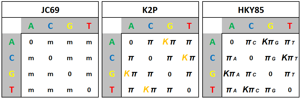
[Left] The original and simplest model is the Jukes & Cantor (1969) model, called JC69, which assumes that all nucleotide frequencies are equal, and all mutations leading to a SNP occur at the same rate, m. For example, the reciprocal rates A C and C A are equal, and equal to A ↔ G. At the time it was introduced, there were few data to suggest otherwise, and more important, the model was mathematically and computationally simple prior to the days of PCs.

[Middle] A simple adjustment is the Kimura Two-Parameter Model (K2P), which recognized from early DNA data that, at least in comparisons within species and among closely-related species, transitions (Ts) (A ↔ G and C ↔ T) are much more frequent than transversions (Tv) (all other pairwise mutations). This is calculated as the Transition Bias (K) [Ts] / [Tv]. As sequence divergences increase, [Tv] increases towards K < 1, and Tv-only models may be more accurate. [This occurs because Ts back mutations (a g a "flip-flops") occur so rapidly that their current state between any two sequences is uninformative. Slower Tv mutations then provide more information].

[Right] Given the availability of data and increased understanding of molecular evolution, it became apparent that besides the Transition Bias, nucleotide frequencies in either DNA strand are unequal, and that mutation rates between nucleotide pairs are unequal. The Hasegawa, Kishino, & Yano (1985) model (HKY85) incorporates all these factors. In the last column, for example, the mutation rate of any nucleotide A, C, or G to T is the same (π_T), except that the rate of transitions CT is weighted by K as in the previous mode. Every other column has the same arrangement.

[Below] Advanced Methods: As computational power and extensive data became available, it is now possible to construct a universal model, called the General Time Reversible (GTR) model, which allows all available information to be incorporated into any particular evolutionary investigation. Estimates of mutation rates are calculated from the data themselves. In the last column, for example, πγ in the HKY95 model is weighted by three different nucleotide-specific factors, ϒ, $ϵ$ η, where η incorporates the Transition Bias. The probability that a base remains unchanged is also explicitly calculated, as the negation of the sum of probabilities in the rest of the row that it does change. Such a probability might be modified by a Poisson correction for multiple hits (a g a). The GTR was previously prohibitively machine-time intensive, and remains so if it has to be re-calculated for each bootstrap replication. A heuristic solution is to use the same estimated GTR matrix for all bootstraps.

${\displaystyle Q={\begin{pmatrix}{-(\alpha \pi _{G}+\beta \pi _{C}+\gamma \pi _{T})}&{\alpha \pi _{G}}&{\beta \pi _{C}}&{\gamma \pi _{T}}\\{\alpha \pi _{A}}&{-(\alpha \pi _{A}+\delta \pi _{C}+\epsilon \pi _{T})}&{\delta \pi _{C}}&{\epsilon \pi _{T}}\\{\beta \pi _{A}}&{\delta \pi _{G}}&{-(\beta \pi _{A}+\delta \pi _{G}+\eta \pi _{T})}&{\eta \pi _{T}}\\{\gamma \pi _{A}}&{\epsilon \pi _{G}}&{\eta \pi _{C}}&{-(\gamma \pi _{A}+\epsilon \pi _{G}+\eta \pi _{C})}\end{pmatrix}}}$

where there are six distinct reciprocal mutation rates:

${\displaystyle {\begin{aligned}\alpha =r(A\rightarrow G)=r(G\rightarrow A)\\\beta =r(A\rightarrow C)=r(C\rightarrow A)\\\gamma =r(A\rightarrow T)=r(T\rightarrow A)\\\delta =r(G\rightarrow C)=r(C\rightarrow G)\\\epsilon =r(G\rightarrow T)=r(T\rightarrow G)\\\eta =r(C\rightarrow T)=r(T\rightarrow C)\end{aligned}}}$